APMR
Acoustical Porous Material Recipes

Section: Home | Basics of Mechanics

Accuracy limits of plate theories

Plate theories (such as Love-Kirchhoff, Reissner-Mindlin theories etc.) are commonly used in many structural and vibroacoustic applications. Therefore, applicability limits of these theories gain a particular interest, especially in acoustic applications, to avoid any mistakes in the design of acoustic packages which might arise from not satisfying the assumptions of these theories in a particular frequency range.

Although qualitative and approximate frequency limits are given in the literature, it is often a tedious task to find an analytical expression for applicability limits. In this aspect, this page discusses the accuracy limits derived for plate theories through analysis of the propagating wavenumbers and admittances of the investigated panels. The following content has been published in:
Arasan U., Marchetti F., Chevillotte F., Tanner G., Chronopoulos D. and Gourdon E., 2021, "On the accuracy limits of plate theories for vibro-acoustic predictions", Journal of Sound and Vibration, 493, p. 115848
(published version or preprint version)
and is discussed in Arasan's PhD defense:

Dispersion relations

Let us consider an infnitely extended elastic plate layer with thickness $h$ (as shown below). For our study, we assume the case where an oblique plane wave impinging on an infinitely extending elastic isotropic plate layer with incident angle $\theta$. This oblique plane wave has the transverse component (or $x$ component) as \[ k_t=k_0\sin\theta, \] where $k_0=\omega/c_0$ is the wavenumber in free air, $\omega=2\pi f$ is the circular frequency of the incident wave and $c_0$ is the speed of sound in air.

For Love-Kirchoff plates (or thin plates), the free vibration analysis would yield the following dispersion relation: \[ k_p^4 D-m_s\omega^2=0\;\;\;\Rightarrow k_p=\textcolor{red}{k_b=\sqrt{\omega\sqrt{\frac{m_s}{D}}}}, \] where $k_b$ corresponds to the bending wavenumber and $k_p$ is the natural propagating wavenumber of the plate. Note that $m_s=\rho h$ is the mass per unit area of the plate while $\rho$ being the density and $D$ is the bending stiffness of the plate (expressed as below). \[ D=\frac{E(1+\text{j}\eta)h^3}{12(1-\nu^2)}, \] where $E$ is the Young's modulus, $\eta$ is the damping/loss factor of the material, $\nu$ is the Poisson's ratio and $\text{j}=\sqrt{-1}$.

For Reissner-Mindlin plates (or thick plates), the free vibration analysis would yield the following dispersion relation: \[ k_p^4 D-m_s\omega^2-k_p^2\frac{Dm_s}{G^{*}h}\omega^2=0. \] Note that the above dispersion relation ignores the membrane effect of the plate as its influence is small compared to the bending and shear effects.
Out of the four solutions, the following wavenumber is always propagative: \[ k_p=k_\text{thick}=\sqrt{\frac{m_s\omega^2}{2G^{*}h}+\sqrt{\frac{m_s\omega^2}{D}+\bigg(\frac{m_s\omega^2}{2G^{*}h}\bigg)^2}}. \] Considering the definition of shear wavenumber ($k_s$) of the plate, the above propagating wavenumber can be written in a compact form as: \[ \textcolor{blue}{k_\text{thick}}=\sqrt{\frac{1}{2}\left[\textcolor{green}{k_s}^2+\sqrt{4\textcolor{red}{k_b}^4+\textcolor{green}{k_s}^4}\right]};\;\;\text{where}\;\;\textcolor{green}{k_s=\frac{m_s\omega^2}{G^{*}h}}. \] $G^{*}=\kappa G$ in the above equations represents the shear modulus ($G$) corrected with the shear correction factor ($\kappa$).

The following interactive application shows the propagating wavenumbers obtained from thin and thick plate theories. You could see the effects each plate properties on the dispersion curves by changing its values below.

Observations:

$\bullet$ At low frequencies, $k_\text{thick}$ approaches the bending wavenumber ($k_b$) given by thin plate theory
$\bullet$ At high frequencies, $k_\text{thick}$ approaches the corrected shear wavenumber ($k_s$)

Frequency limits of plate theories

Limit for thin plate (Love-Kirchhoff) theory:
Following the above-mentioned observations, we could formulate a condition, $k_b\ge C_kk_s$, to find the frequency limit of thin plate theory. The value of $C_k$ must be chosen in such a way that the error between the values of $k_\text{thick}$ and $k_b$ is below 5%.
The relation between the error percentage and $C_k$ can be found in page 8 (Eqs. 18 and 19) of this article.

The frequency limit expression for thin plate theory is then expressed as follows from the condition between the bending and shear wavenumbers: \[ k_b\geq C_kk_s\Rightarrow f\leq f_{\textrm{thin/thick}}=\displaystyle\frac{G^{*}h}{2\pi C_k^2}\sqrt{\displaystyle\frac{1}{m_sD}}=\displaystyle\frac{\kappa}{4\pi hC_k^2}\sqrt{\displaystyle\frac{12E}{\rho}\displaystyle\frac{1-\nu}{1+\nu}} \] where $f_{\textrm{thin/thick}}$ is the frequency limit of the 'thin' plate theory by keeping the 'thick' plate theory as reference. Note that for a typical isotropic layer, $C_k=4$ can be chosen which corresponds to 2% error between $k_\textrm{thick}$ and $k_b$.

Limit for plate theory in general:
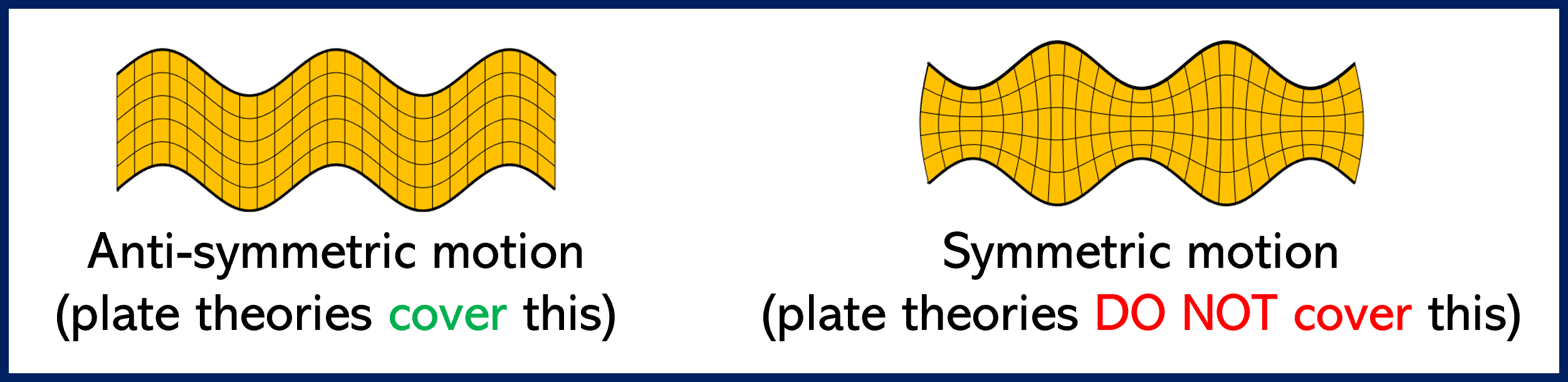
Since the most commonly used plate thoeries (Love-Kirchhoff, Reissner-Mindlin etc.) do not include the displacement field correspond to the symmetric motion of the plate, comparing the admittances (or impedances) of the anti-symmetric and symmetric motions of the structure would be a possible way to find the frequency limit of plate theories.
The impedance correspond to anti-symmetric motion can be expressed as (from thin plate theory): \[ Z_\text{A}=\frac{1}{Y_A}=\text{j}\omega m_s\bigg(1-\displaystyle\frac{Dk_t^4}{\omega^2 m_s}\bigg). \] The approximate impedance correspond to symmetric motion can be expressed as (from Transfer Matrix Method (TMM)): \[ Z_\text{S}=\frac{1}{Y_S}=\displaystyle\frac{4K}{\text{j}\omega h}, \] where $K=\lambda+2\mu$ is the compressional modulus of the elastic layer and $\lambda,\mu$ are Lamé coefficients. The limit for plate theory is then could be computed by defining a condition as follows: \[ \left|\frac{Z_S}{Z_A}\right|=\left|\frac{Y_A}{Y_S}\right|\geq C_y \Rightarrow f\leq f_{\mathrm{{plate/solid}}}=\displaystyle\frac{c_0^2}{2\pi\sin^2\theta}\sqrt{\displaystyle\frac{m_s}{2D}\pm\sqrt{\left(\displaystyle\frac{m_s}{2D}\right)^2\pm\displaystyle\frac{4K}{hC_yD}\displaystyle\frac{\sin^4\theta}{c_0^4}}}. \] Note:
$\bullet$ The subscript 'plate/solid' in the above equations means that the frequency limit is for 'plate' theories in general (as even higher order plate theories also do not account for symmetric motion) by keeping as a reference the theory of 'elastic solids (or TMM)'.

$\bullet$ Although the above expression is applicable for any angle of incidence, it would be practical to use $\sin\theta=1$ to cover for the diffuse field excitation.

$\bullet$ $C_y=10$ is suitable for most practically used isotropic plates.

$\bullet$ Out of four values, minimum of two pure real roots is taken to be the value for frequency limit.

$\bullet$ One could use impedance from Reissner-Mindlin plate theory to find the expression for $f_{\mathrm{{plate/solid}}}$. However, it is observed that Love-Kirchhoff theory also provides good approximation.

Unless otherwise indicated, the content of this page is copyleft under :
the creative commons license Attribution 3.0 Unported (CC BY 3.0),
Arasan Uthayasuryian & Luc Jaouen (@ljaouen), ISSN 2606-4138.
Site hosted by Matelys.