This page is a complementary material to the paper "Length correction of 2D discontinuities or perforations at large wavelengths and for linear acoustics" authored by Luc Jaouen & Fabien Chevillotte and published in Acta Acustica United with Acustica in March 2018 (Vol. 104(2) pp. 243 – 250). An open access version is available on Arxiv.
The length correction for acoustic radiation
A first approximation when studying duct opening in an open plane is to set the acoustic pressure equal to 0 at the aperture (stating that the pressure field is continuous and the pressure at the aperture should equal the pressure far from the duct aperture, i.e. 0).
This approximation of the position of the first acoustic node is not accurate enough when one wants to design the pipes of a pipe organ or when one wants to predict the sound absorption of a perforated plate.
A better estimation of the note generated from the pipe or of the position in frequency of the absorption peak of a perforated plate relies on calculating the length correction related to the radiation effect : $\varepsilon$.
The most common values of the length corrections are probably the ones for a semi-infinite duct radiating in the half plane (first scheme below) :
\[
\varepsilon_{0}^{\textrm{long duct, baffled, piston motion}} = \frac{8r}{3 \pi} \simeq 0.85 r
\]
and the one of a semi-infinite duct radiating in the open plane (second scheme below) :
\[
\varepsilon_{0}^{\textrm{long duct, unbaffled}} = 0.62 r
\]
These expressions are based on assumptions described in e.g.
Jaouen & Chevillotte 2018. The origins of other expressions such as $\varepsilon_{0}^{\textrm{long duct, baffled}} = 0.82 r$ are also discussed in this publication.
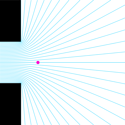
Case of the 2D flanged duct (a semi-infinite duct, on the left, opens in the half plane on the right; the infinitely-long and thick flanged is depicted by the black rectangles $\blacksquare$). The blue lines ($\textcolor{#00ccFF}{\boldsymbol{-}}$) denote the streamlines. The pink bullet ($\textcolor{#ff00cc}{\bullet}$) denotes the first acoustic pressure node outside the duct. The length correction is the distance between the aperture and this first pressure node.
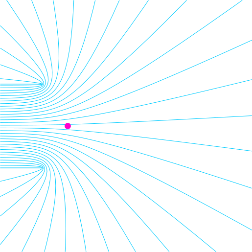
Case of the 2D unflanged duct (a semi-infinite duct, on the left, opens in the open plane). The blue lines ($\textcolor{#00ccFF}{\boldsymbol{-}}$) denote the streamlines. The pink bullet ($\textcolor{#ff00cc}{\bullet}$) denotes the acoustic pressure node outside the duct. Again, the length correction is the distance between the aperture and this first pressure node.
In the plots above (and below), the streamlines ($\textcolor{#00ccFF}{\boldsymbol{-}}$) are the paths followed by fluid particles in case of flow. For an acoustic excitation, the particles oscillate along an equilibrium position following these streamlines.
A plethora of equations (one for each different geometry)
The specific cases above, studied by H. von Helmholtz or J. W. Strutt, do not address the geometry of the duct cross-section (the duct openings have a characteristic dimension - their radii - very small compared to the other dimensions).
Since 1941 and the works by V. A. Fok (В. A. Фок) and V. S. Nesterov (В. С. Нестеров), a plethora of studies, and equations, have been published to estimate the value of the length correction (
see the Arxiv's version of Jaouen & Chevillotte for full references). Each equation being dedicated to a specific geometry as depicted with the 3D objects below (click/tap and drag to change perspective).
Circular tube opening in a larger square tube. U. Ingard fisrt solves this case providing an expression for $\varepsilon_{\circ\subset\blacksquare}$. His derivation is reported below.
Circular tube opening in a larger square tube. Again, U. Ingard first solves this case providing an expression for $\varepsilon_{\square\subset\blacksquare}$. His derivation is reported below.
What is a general expression for the length correction for a duct with an arbitrary cross-section opening in a larger duct with another arbitrary cross-section ? This is the question discussed in the section below.
But one single formula can rule them all (almost)
For the case of a duct discontinuitiy (between 2 coaxial ducts) or a straight and centered perforation (with respect
to a pattern), Jaouen & Chevillotte found out that all previous (and correct) published works give the same results if plotted against the surface ratio at the duct discontinuity or the perforation ratio (two descriptions denoting the same variable written hereafter as $\phi$).
The expression of the length correction derived in Jaouen & Chevillotte is :
\[
\varepsilon \simeq \varepsilon_0 \Big( 1-1.33\sqrt{\phi}-0.07\sqrt{\phi}^2+0.40\sqrt{\phi}^3 \Big)
\]
where the value for $\varepsilon_0$ is given, as a first approximation, by $0.85 r$ or $0.82 r$ (see top of this page) but a refined expression of $\varepsilon_0$ can be used if the duct has a lateral characteristic dimension (the radius for a duct with a circular cross-section) which is not much smaller than the length of the duct (see section 4 of the article).
Formulas by Fok, Nesterov, Kergomard & Garcia, Jaouen & Bécot can also be applied as long as they are written as functions of $\sqrt{\phi}$ (see references and expressions in Jaouen & Chevillotte)
The plot on the left (or above) shows the streamlines and the first acoustic pressure node for a duct discontinuity with a surface ratio (or perforation rate) of $\phi$ = .
Drag the numerical value to change $\phi$ and see the effect on the streamlines and on the length correction.
Nota Bene :
$\bullet$ The plot corresponds to a 2D projection of a circular duct inside a larger circular duct or a square duct inside a larger square duct.
$\bullet$ The change in length correction (between the duct discontinuity and the acoustical node) from one computation to another is not straight forward as both $\phi$ and the radius (or the edge for a square cross-section) change between computations.
Additional derivations
Here, we derive the expressions of the length corrections, as presented by Uno Ingard (in "On the Theory and Design of Acoustic Resonators", J. Acoust. Soc. Am. 25, 1953, 1037-1061
DOI), for a rectangular perforation in a rectangular pattern and a circular perforation in a rectangular pattern.
The perforation schemes and the nomenclature used are the ones reported in the figures below.
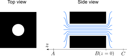

The length corrections derived here, $\varepsilon$, are determined by calculating the impedances at $z=0$ and at low pulsations $\omega$, seen by a wave propagating towards $z>0$.
This impedances writes (see e.g. [Ray45],[Ing53b]):
\[
Z_{B} = \bar{p} / U_0 = \phi Z_0 - j\omega \rho_0 \varepsilon
\]
$\bar{p}$ is the mean value of the pressure over the perforation surface area while $U_0$ is, following J. W. Strutt's first assumption (J. W. Strutt aka 3rd lord Rayleigh, The theory of sound, volume 2, second edition, Macmillan & Co. Ltd. New York, 1896, Appendix A, pp. 487-491), the uniform velocity amplitude of the particle velocity over the perforation surface area, i.e. the particle motion is assumed to be a piston-like motion with $\varepsilon_{0}$ being given by: $\varepsilon_{0}^{\textrm{constant},\ h>r} = 8/(3 \pi^{3/2}) \sqrt{A_0}$}. $Z_0$ is the characteristic impedance of the air: $Z_0=\rho_0 c_0$ where $\rho_0$ is the mass density of air at rest ($\sim$ 1.2 kg.m$^{-3}$) and $c_0$ is the speed of sound in the air ($\sim$ 340 m.s$^{-1}$).
Rectangular perforation in a rectangular pattern
Due to perforation periodicity, the velocity components in the same planes as the interfaces between two patterns should be equal to zero. Thus, a wave propagating towards $z>0$ appears to propagates in a rectangular waveguide with the dimensions of the pattern: $2a \times 2b$.
The expression of the pressure field in the Representative Elementary Volume (REV) for $z>0$ is given by:
\[
p(x,y,z)=\sum_{m}\sum_{n}{P_{mn} \cos\left(\frac{\pi m x}{a}\right) \cos\left(\frac{\pi n y}{b}\right) e^{-jk_{mn}z}}
\]
where the expression of the wavenumber magnitude for mode ($m,n$) is:
\[
k_{mn}=\sqrt{k^2-k_x^2-k_y^2}
\]
with
\[
k=\omega/c_0 , \ k_x=\frac{m\pi}{a}\ \textrm{and}\ k_y=\frac{n\pi}{b}
\]
The expression for the z-component of the particle velocity, $u_z$, is deduced from Euler's equation:
\[
u_z(x,y,z)=\sum_{m}\sum_{n}{U_{mn} \cos\left(\frac{\pi m x}{a}\right) \cos\left(\frac{\pi n y}{b}\right) e^{-jk_{mn}z}}
\]
where
\[
U_{mn}=\frac{k_{mn} P_{mn}}{\omega\rho_0}
\]
Considering a uniform velocity amplitude of the particle velocity over the perforation (i.e. piston-like motion), $U_0$, the normal velocity at $z=0$ is written:
\[
u_z\left(x,y,0\right)=d\left(x,y\right) U_0=\sum_{m,n}U_{mn} \cos\left(\frac{\pi m x}{a}\right) \cos\left(\frac{\pi n y}{b}\right)
\]
where $d(x,y)$ is the distribution function equal to 1 for $-a_1\leq x\leq a_1$ and $-b_1\leq y\leq b_1$, while $d(x,y)=0$ everywhere else.
To express $U_{mn}$, the last equation is multiplied by $\cos(\pi m x/a) \cos(\pi n y/b)$ and integrated over the cross-section of the REV:
\[
\begin{aligned}
\int^{a}_{-a}\int^{b}_{-b}d(x,y) U_0 \cos\left(\frac{\pi m x}{a}\right) \cos\left(\frac{\pi n y}{b}\right)dxdy&=\\ \int^{a}_{-a}\int^{b}_{-b} \sum_{m',n'}U_{m'n'} \cos\left(\frac{\pi m' x}{a}\right) \cos\left(\frac{\pi n' y}{b}\right)\cos\left(\frac{\pi m x}{a}\right) \cos\left(\frac{\pi n y}{b}\right)dxdy &
\end{aligned}
\]
Using the orthogonality property of modes $\cos(\pi m x/a) \cos(\pi n y/b)$, one writes:
\[
\begin{aligned}
\int^{a_1}_{-a_1}\int^{b_1}_{-b_1} U_0 \cos\left(\frac{\pi m x}{a}\right) \cos\left(\frac{\pi n y}{b}\right)dxdy &=
\int^{a}_{-a}\int^{b}_{-b} U_{mn} \cos^2\left(\frac{\pi m x}{a}\right) \cos^2\left(\frac{\pi n y}{b}\right)dxdy \\
4 U_0 \frac{ab}{\pi^2mn} \sin\left(\frac{\pi m a_1}{a}\right) \sin\left(\frac{\pi n b_1}{b}\right)
&= U_{mn} \frac{ab}{\nu_{mn}}
\end{aligned}
\]
where $\nu_{00}=1/4$, $\nu_{0n}=\nu_{m0}=1/2$ and $\nu_{mn}=1$ when $m\neq0$ and $n\neq0$.
$U_{mn}$ now writes:
\[
U_{mn}=4 \nu_{mn} U_0 \frac{\sin\left(\pi m \xi\right) \sin\left(\pi n \eta\right)}{\pi^2mn}
\]
where two dimensionless shape ratios have been introduced: $\xi=a_1/a$ and $\eta=b_1/b$ (the product $\xi\eta$ is thus equal to the perforation rate $\phi$).
From what's above, $P_{mn}$ writes:
\[
P_{mn}=\frac{4 \nu_{mn} \omega\rho U_0}{k_{mn}} \frac{\sin(\pi m \xi) \sin(\pi n \eta)}{\pi^2 m n}
\]
The mean value for the pressure over the perforation surface area, $\bar{p}$, is obtained integrating the equation of the pressure over this perforation:
\[
\bar{p}=\frac{1}{4a_1b_1}\int^{a_1}_{-a_1}\int^{b_1}_{-b_1}\sum_{mn}P_{mn}\cos\left(\frac{\pi m x}{a}\right) \cos\left(\frac{\pi n y}{b}\right)dxdy
\]
\[
\bar{p}=\frac{1}{4a_1b_1}\sum_{mn}\frac{16 \nu_{mn} \omega\rho_0 U_0}{k_{mn}} \xi \eta a_1 b_1 \left[\displaystyle\frac{\sin(\pi m \xi)}{\pi m \xi} \frac{\sin(\pi n \eta)}{\pi n \eta}\right]^2
\]
\[
\bar{p}=\sum_{mn}\frac{4\nu_{mn} \omega\rho_0 U_0}{k_{mn}} G_{mn}
\]
with
\[
G_{mn}= \Big[\frac{\sin(\pi m \xi)}{\pi m \xi} \frac{\sin(\pi n \eta)}{\pi n \eta}\Big]^2 (\xi\eta)
\]
At low frequencies, $\omega \ll \omega_{mn}$, $k_{mn}$ values can be approximated with:
\[
k_{mn}\approx\sqrt{-\left(k_x^2+k_y^2\right)}\approx j\sqrt{\left(\frac{m\pi}{a}\right)^2+\left(\frac{n\pi}{b}\right)^2}
\]
The expression of the end correction $\varepsilon$ is obtained from expression of the impedance $Z_B$.
\[
\varepsilon_{\Box\subset\blacksquare} =\frac{4}{\pi}\sum_{mn^*}\frac{\nu_{mn}G_{mn}}{\sqrt{\left(\displaystyle\frac{m}{a}\right)^2+\left(\displaystyle\frac{n}{b}\right)^2}}
\]
$\sum_{mn^*}$ indicates a sum over $m$ and $n$ where the mode ($m=0$, $n=0$) is not accounted for (this mode contributes to the real part of the impedance $Z_{B}$).
Circular perforation in a rectangular pattern
The derivation presented in the section section is now applied for a circular perforation in a rectangular pattern. For this second configuration, the normal velocity at $z = 0$ writes:
\[
u_z(x,y,0)=d\left(x,y\right) U_0 = \sum_{m,n}U_{mn} \cos\left(\frac{\pi m x}{a}\right) \cos\left(\frac{\pi n y}{b}\right)
\]
where the distribution function $d(x,y)$ equals $1$ for $r=\sqrt{x^2+y^2}\leq r_1$ and $0$ everywhere else.
The expression of $u_z(x,y,0)$ is multiplied by $\cos(\pi m x/a) \cos(\pi n y/b)$ and integrated over the perforation surface area. Finally, using the orthogonality property of modes $\cos(\pi m x/a) \cos(\pi n y/b)$ and the polar coordinates system, one can write:
\[
\begin{aligned}
\int^{2\pi}_{0}\int^{r_1}_{0} U_0 \cos\left(\frac{\pi m r \cos(\theta)}{a}\right) \cos\left(\frac{\pi n r \sin(\theta)}{b}\right)rdrd\theta \\
= \int^{a}_{-a}\int^{b}_{-b} U_{mn} \cos^2\left(\frac{\pi m x}{a}\right) \cos^2\left(\frac{\pi n y}{b}\right)dxdy
\end{aligned}
\]
The oscillatory part of the left hand side in the previous equation can be re-written as:
\[
\begin{aligned}
&\cos\left(\frac{\pi m r \cos(\theta)}{a}\right) \cos\left(\frac{\pi n r \sin(\theta)}{b}\right)\\
&=\frac{1}{2}\cos\left(r\sqrt{\displaystyle\left(\frac{\pi m}{a}\right)^2+\left(\frac{\pi n}{b}\right)^2}\sin\left(\theta+\gamma\right)\right)\\
&+\frac{1}{2}\cos\left(r\sqrt{\displaystyle\left(\frac{\pi m}{a}\right)^2+\left(\frac{\pi n}{b}\right)^2}\sin\left(\theta-\gamma\right)\right)
\end{aligned}
\]
with $\gamma=\arctan{\displaystyle\left(\frac{na}{mb}\right)}$.
Using
\[
\int_{0}^{2\pi}\cos\left(r\sqrt{\displaystyle\left(\frac{\pi m}{a}\right)^2+\left(\frac{\pi n}{b}\right)^2}\sin\left(\theta\pm\gamma\right)\right)=2\pi J_0\left(r\sqrt{\displaystyle\left(\frac{\pi m}{a}\right)^2+\left(\frac{\pi n}{b}\right)^2}\right)
\]
and the property of Bessel functions of the first kind: $\int_{0}^{X} J_0(x)xdx=XJ_1(X)$, one writes:
\[
\begin{aligned}
&\int_{0}^{r_1}J_0\left(r\sqrt{\displaystyle\left(\frac{\pi m}{a}\right)^2+\left(\frac{\pi n}{b}\right)^2}\right)rdr\\
&=\int_{0}^{r_1'}J_0\left(r'\right)\displaystyle\frac{r'dr'}{\left(\displaystyle\frac{\pi m}{a}\right)^2+\left(\displaystyle\frac{\pi n}{b}\right)^2}\\
&=r_1 \frac{J_1\left(r_1\sqrt{\displaystyle\left(\frac{\pi m}{a}\right)^2+\left(\frac{\pi n}{b}\right)^2}\right)}{\sqrt{\displaystyle\left(\frac{\pi m}{a}\right)^2+\left(\frac{\pi n}{b}\right)^2}}
\end{aligned}
\]
so that the double integration equation now writes:
\[
2\pi r_1 U_0 \frac{J_1\left(r_1\sqrt{\displaystyle\left(\frac{\pi m}{a}\right)^2+\left(\frac{\pi n}{b}\right)^2}\right)}{\sqrt{\displaystyle\left(\frac{\pi m}{a}\right)^2+\left(\frac{\pi n}{b}\right)^2}}=U_{mn} \frac{ab}{\nu_{mn}}
\]
$U_{mn}$ and $P_{mn}$ can be expressed as:
\[
U_{mn}=\frac{2\pi r_1 \nu_{mn} U_0}{ab} \frac{J_1\left(r_1\sqrt{\displaystyle\left(\frac{\pi m}{a}\right)^2+\left(\frac{\pi n}{b}\right)^2}\right)}{\sqrt{\displaystyle\left(\frac{\pi m}{a}\right)^2+\left(\frac{\pi n}{b}\right)^2}}
\]
and
\[
P_{mn}=\frac{2\pi r_1 \nu_{mn} U_0}{ab}\frac{\rho \omega}{k_{mn}} \frac{J_1\left(r_1\sqrt{\displaystyle\left(\frac{\pi m}{a}\right)^2+\left(\frac{\pi n}{b}\right)^2}\right)}{\sqrt{\displaystyle\left(\frac{\pi m}{a}\right)^2+\left(\frac{\pi n}{b}\right)^2}}
\]
The mean pressure over the perforation area $\bar{p}$ writes:
\[
\bar{p}=\frac{1}{\pi r_1^2}\int_{0}^{2\pi}\int_{0}^{r_1}\sum_{mn}P_{mn}\cos\left(\frac{\pi m r \cos(\theta)}{a}\right) \cos\left(\frac{\pi n r \sin(\theta)}{b}\right)rdrd\theta
\]
\[
\bar{p}=\frac{1}{\pi r_1^2}\sum_{mn}\frac{4\pi^2 r_1^2 \nu_{mn} U_0}{ab}\frac{\rho \omega}{k_{mn}} \left[\frac{J_1\left(r_1\sqrt{\displaystyle\left(\frac{\pi m}{a}\right)^2+\left(\frac{\pi n}{b}\right)^2}\right)}{\sqrt{\displaystyle\left(\frac{\pi m}{a}\right)^2+\left(\frac{\pi n}{b}\right)^2}}\right]^2
\]
From the approximate expression for $k_{mn}$ recalled in the previous section:
\[
\bar{p}=\frac{4\pi}{ab} U_0 \rho \omega\sum_{mn}\nu_{mn} \frac{J_1^2\left(r_1\sqrt{\displaystyle\left(\frac{\pi m}{a}\right)^2+\left(\frac{\pi n}{b}\right)^2}\right)}{j\left[\displaystyle\left(\frac{\pi m}{a}\right)^2+\left(\frac{\pi n}{b}\right)^2\right]^{3/2}}
\]
Finally, from the expression of the impedance $Z_B$, the expression of the length correction $\varepsilon_{\circ\subset\blacksquare}$ is derived:
\[
\varepsilon_{\circ\subset\blacksquare}=\frac{4\pi}{ab} \sum_{mn*} \nu_{mn} \frac{J_1^2\left(r_1\sqrt{\displaystyle\left(\frac{\pi m}{a}\right)^2+\left(\frac{\pi n}{b}\right)^2}\right)}{\left[\displaystyle\left(\frac{\pi m}{a}\right)^2+\left(\frac{\pi n}{b}\right)^2\right]^{3/2}}
\]
For this configuration, the shape ratios $\xi$ and $\eta$ are re-defined as $r_1/a$ and $r_1/b$ respectively.