The potential flow around a circular cylinder is a classical problem studied in fluid mechanics. From its solution, some other problems can be studied, such as the flow around the wing of a plane with a more realistic airfoil.
In this simple example, a wing is modeled as an infinite cylinder, transverse to a uniform and unidirectional flow. The fluid is supposed to be inviscid and incompressible.
This animation shows the streamlines around the gray disk (or infinite cylinder in 3D) of a uniform and unidirectional (on the left hand side), inviscid and incompressible flow. Differences in lengths of the streamlines are observed, but all particles begin at the same time on the left side and arrive at the same time on the right side for the particular case studied here (this is not the case with most real-life experiments).
A first mathematical derivation
A disk (or a cylinder in 3D) of radius $R$ is placed in a two-dimensional (or three-dimensional), incompressible, inviscid, uniform flow.
The goal is to find the steady velocity vector $\mathbf{V}$ and pressure $p$ in a plane, subject to the condition that far from the cylinder the velocity vector is :
\[
\mathbf{V} = U\mathbf{e_x}+0\mathbf{e_y}
\]
where $\mathbf{e_x}$ and $\mathbf{e_y}$ are the unit vectors of the $x$ and $y$ axes and where $U$ is a constant.
At the boundary of the cylinder :
\[
\mathbf{V}\cdot\mathbf{\hat n}=0
\]
where $\mathbf{\hat n}$ is the vector normal to the cylinder surface.
The upstream flow is uniform and has no vorticity. The flow is inviscid, incompressible and has a constant mass density $\rho$. Thus, the flow remains without vorticity (or is said to be irrotational, i.e. $\nabla\times \mathbf{V} = 0$) everywhere.
As an irrotational flow, there must exist a velocity potential $\phi$ :
\[
\mathbf{V}=\nabla\phi
\]
As an incompressible fluid (i.e. $\nabla\cdot \mathbf{V} = 0$), $\phi$ must satisfy Laplace's equation :
\[
\nabla^2\phi=0
\]
The solution for $\phi$ is obtained most easily in polar coordinates $r$ and $\theta$, related to the Cartesian coordinates by $x=r\cos\theta$ and $y=r\sin\theta$.
In polar coordinates, Laplace's equation is rewritten :
\[
\frac{1}{r}\frac{\partial}{\partial r}\left(r \frac{\partial \phi}{\partial r}\right) + \frac{1}{r^2}\frac{\partial^2 \phi}{\partial \theta^2} = 0
\]
The solution that satisfies the boundary conditions is :
\[
\phi(r,\theta)=Ur\left(1+\frac{R^2}{r^2}\right)\cos\theta
\]
The velocity components in polar coordinates are obtained from the components of $\nabla \phi$ in polar coordinates:
\[
V_r=\frac{\partial \phi}{\partial r} = U\left(1-\frac{R^2}{r^2}\right)\cos\theta
\]
and
\[
V_\theta=\frac{1}{r}\frac{\partial \phi}{\partial \theta} = - U\left(1+\frac{R^2}{r^2}\right)\sin\theta
\]
Being invisicid and irrotational, Bernoulli's equation allows the solution for pressure field to be obtained directly from the velocity field. Here it takes the form :
\[
p=\frac{1}{2}\rho\left(U^2-V^2\right) + p_\infty
\]
where $p_\infty$ is the pressure far from the cylinder (where $\mathbf{V} = U\mathbf{e_x}$) and $|\mathbf{V}|^2 = V^2$. Using $V^2=V_r^2+V_{\theta}^2$ :
\[
p=\frac{1}{2}\rho U^2\left(2\frac{R^2}{r^2}\cos(2\theta)-\frac{R^4}{r^4}\right) + p_\infty
\]
In the figures, the colorized field, referred to hereafter as the "normalized pressure", is a plot of :
\[
2 \frac{p - p_\infty}{\rho U^2} =2\frac{R^2}{r^2}\cos(2\theta)-\frac{R^4}{r^4}
\]
The flow being incompressible, a stream function can be found such that
\[
\mathbf{V}=\nabla\psi \times \mathbf{e_z}
\]
It follows from this definition, using vector identities :
\[
\mathbf{V}\cdot\nabla{\psi}=0
\]
Therefore, a contour of a constant value of $\psi$ will also be a streamline, a line tangent to $\mathbf{V}$. For the flow past a cylinder, we find :
\[
\psi= U \left( r - \frac{R^2}{r} \right) \sin\theta
\]
"Normalized pressure" in color (red is maximum : +1, blue is minimum : -3), streamlines as animated dashed black curves and equipotentials (curves of equal velocity potential) in white for the non-viscid flow around a disk (or an infinite cylinder in 3D). This animation is heavily inspired from a static picture by Wikipedia's contributor Incredio in the page discussing the same topic on Wikipedia.
Below are four observations or comments about the results above.
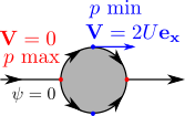
Two points have a zero velocity : ($R$,$\theta=0$) and ($R$,$\theta=\pi$). They are called stagnation points. At these points, the "normalized pressure" is maximum and equals 1.
The two points ($R$,$\theta=\pi/2$) and ($R$,$\theta=3\pi/2$) have a velocity $\mathbf{V} = 2U\mathbf{e_x}$. At these points, the "normalized pressure" is minimum and equals -3.
These 4 previous points belong to the particular streamline $\psi = 0$ which corresponds to the axis $y=0$ outside the disk of radius $R$ and the perimeter of this disk (composed by the two top and bottom half circles).
Scheme illustrating the streamline $\psi=0$ to which belong the two stagnation points (in red) and the two points with a maximum velocity along the $x$ axis (in blue).
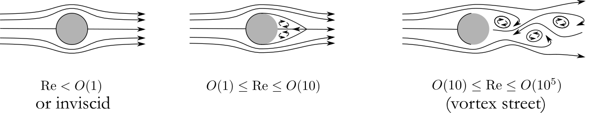
The symmetry of the problem with respect to the $x$ and $y$ axes implies this model can't explain, respectively, drag and lift forces observed when the fluid is viscous. For a viscous fluid and a Reynolds number, Re, on the order of 1 and above, a thin boundary layer at the surface of the cylinder will occur. This implies, in turn, a trailing wake in the flow behind the cylinder. The symmetry with respect to the $y$ axis will be lost and the pressure at each point on the wake side of the cylinder will be lower than on the upstream side, resulting in a drag force in the downstream direction.
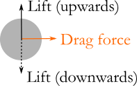
The $x$-axis symmetry is also lost when considering a viscous fluid (or a rotating cylinder in the case of a inviscid fluid). One can calculate that the average pressure on the upper surface of the cylinder becomes lower (or greater) than the average pressure on the underside. This pressure difference results in an upward (or downward) lift force.
Schemes of the flow for various values of the Reynolds number : Re (ratio of inertial forces to viscous ones). The case studied here is the one of an inviscid fluid (first scheme from the left).
Scheme of the lift and drag forces. The direction (and amplitude) of the lift force depends on multiple parameters (such as the angle of attack, the airfoil profile, the possible rotation of the airfoil...).
A second mathematical derivation using conformal mapping
As we only consider the potential flow problem (i.e. the velocity field can be expressed as the gradient of a scalar function and is thus irrotational), a conformal mapping can be used to solve this Laplace problem ($\nabla^2\phi=0$).
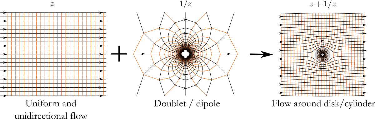
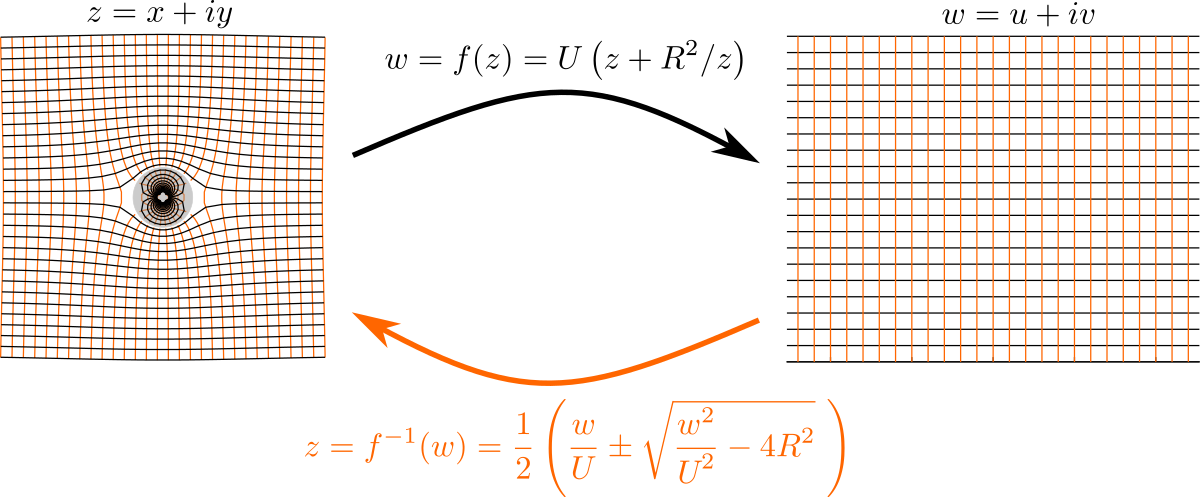
The transformation that maps the uniform and unidirectional flow to the case studied here (of the form $z+1/z$) is :
\[
f(z) = U\left(z+R^2/z\right)
\]
where $z = x+iy$.
This transformation ensures that the celerity of the uniform and unidirectional flow, far from the cylinder, equals $U$.
This transformation corresponds to a uniform and unidirectional flow (first right-hand side term of the form $z$) superposed with a doublet (also called a dipole) i.e. a combination of a source-sink pair of infinite strength kept an infinitesimally small distance apart (second right-hand side term of the form $1/z$). The construction of $f(z)$ might not seem obvious when not used to conformal mapping.
Construction of the conformal mapping of the flow around a disk from a combination of a uniform and unidirectional flow with a doublet (or dipole). Streamlines are in black while equipotentials are in orange. Arrows show the flow direction on some streamlines. Note that the scale and the number of streamlines differ from one plot to another (mainly for the sake of clarity in particular for the doublet). Streamlines and velocity potentials are plotted inside the disk, but they are not considered from a physical point of view.
The velocity potential is obtained as the real part the transformation mapping :
\[
\phi= \Re e \Big[f(x)\Big] = U \left( r + \frac{R^2}{r} \right) \cos\theta
\]
The expression of the streamline function, which is perpendicular to the velocity potential, is obtained as the imaginary part of the transformation mapping :
\[
\psi= \Im m \Big[f(x)\Big] = U \left( r - \frac{R^2}{r} \right) \sin\theta
\]
From the expression of the velocity potential, the velocity can be expressed as well as the pressure using Bernoulli's equation (as derived in the previous section).
Note that the streamlines and equipotentials plotted above (except in the schemes) are obtained from the $w$-space, applying the inverse mapping function $f^{-1}$ :
Relations between the $z$ and $w$ spaces. Both $+$ and $-$ solutions are used to map the $w$-space to the $z$ one (each solution mapping half the $z$-space). Again, streamlines and velocity potentials are plotted inside the disk in the $z$-space. However these "inner" streamlines are not considered from a physical point of view when studying the flow around a disk. The scale and the number of streamlines differ from one plot to another.
Matlab/GNU Octave script
Below is a Matlab/GNU Octave script named FlowAroundADisk.m, which can be used to plot the figures of the streamlines, the equipotentials & the pressure field above.
The streamlines and equipotentials plotted on this page were generated from the conformal mapping (instead of the buil-in "contour" function, based on the "Marching squares" algorithm). The last part of this script shows the example of the conformal mapping applied to plot the streamlines.
% Plot the figures of the streamlines, the equipotentials & the pressure field% for the potential flow around a disk as discussed at :% https://apmr.matelys.com/BasicsMechanics/Fluid/FlowAroundADisk.html% luc.jaouen@matelys.com in Acoustical Porous Media Recipes (ISSN 2606-4138)% Copyleft CC BY 3.0, 2021 %% Enter the 21st century, cite webpage that desserves it.
clear all
close all
%% Constants
U = 20; % Velocity far from disk/cylinder
R = 4; % cylinder radius%% Building the "mesh" used to compute and display the results
x_min = -20; % min x mesh grid results
x_max = 20; % max x
y_min = -20; % min y
y_max = 20; % max y
n = 800; % Number of intervals in grid% Building the mesh on which results will be plotted
[x,y] = meshgrid([x_min:(x_max-x_min)/n:x_max],[y_min:(y_max-y_min)/n:y_max]');
% We set x and y to 0 for points inside the cylinder% thus r = sqrt(x.^2+y.^2) will be 0 and 1/r : NaN % and NaN values are not plotted (they remain white).for i = 1:length(x)
for k = 1:length(x) % mesh is square
f = sqrt(x(i,k).^2 + y(i,k).^2);
if f < R
x(i,k) = 0;
y(i,k) = 0;
endendend%% Computation of the polar variables
r = sqrt(x.^2+y.^2);
sin_th = y./r;
cos_th = x./r;
%% Expression of the velocity potential function
phi = U*r.*(1+R^2./r.^2).*cos_th;
%% Expression of the streamline function
psi = U*r.*(1-R^2./r.^2).*sin_th;
%% Computation & plot of the "normalized pressure"
cos_2th = cos_th.^2 - sin_th.^2;
Twop_pinf2_div_rhoU2 = 2*R^2./r.^2.*cos_2th - R^4./r.^4;
figure(1)
colormap jet
surf(x/R,y/R,Twop_pinf2_div_rhoU2,'EdgeColor','None');
view(2);
grid off
hold on
colorbar
xlabel('x/R')
ylabel('y/R')
title('Normalized pressure')
%% Trick to show a disk at (0,0) with radius R% We'll use this in the next plots.
m = 100;
s = ones(1,m+1)*R;
t = [0:2*pi/m:2*pi];
%% Plot of velocity potentials% We'll use the contour function.% which is based on the Marching squares algorithm.% An alternative is to use Conformal mapping (see end of script).
figure(2)
contour(x,y,phi,50); % 50 is the number of velocity potential curves
hold on
polar(t,s,'k-');
axis equal
title('Velocity potentials');
grid off
%% Plot of streamlines% Again, we'll use the contour function.% An alternative is to use Conformal mapping (see end of script).
figure(3)
contour(x,y,psi,50);
hold on
polar(t,s,'k-');
axis equal
title('Streamlines');
grid off
%% Conformal mapping - for streamlines% The "mesh" is changed for plotting streamlines% 30 streamlines with 30 points along them
n = 30;
m = 30;
figure(4)
hold on
title("z = f(-1)(w=u+iv)")
xlabel("x");
ylabel("y");
for b=1:1:m
v = y_min + (b-1)*(y_max-y_min)/(m-1);
x = zeros(1,n);
y = zeros(1,n);
for a = 1:1:n
u = x_min + (a-1)*(x_max-x_min)/(n-1);
w = u+1j*v;
% At this point, we have created a rectangular map% w = u + iv
signe = -1;
if (u > 0) signe = 1; end
z = 0.5*(w + signe* sqrt(w.^2 -4*R^2));
% Above is f^(-1).% Here, we only care about the position of the points but not% the exact values of the streamlines function so U is taken to 1.
x(a) = real(z);
y(a) = imag(z);
end
plot(x/R,y/R,'k-')
% Mapping the interior of the disk % (just for fun as no physical meaning)for a = 1:1:n
u = x_min + (a-1)*(x_max-x_min)/(n-1);
w = u+1j*v;
signe = 1;
if (u > 0) signe = -1; end
z = 0.5*(w + signe* sqrt(w.^2 -4*R^2));
x(a) = real(z);
y(a) = imag(z);
end
plot(x/R,y/R,'k-')
end
polar(t,s/R,'r-');
axis equal;